Some coming updates

This will be just a short post to show a couple of the new graph types that will be available in the next release of OT/JSvg. Both of them are the result of a project I've been working on for the orthopedics guys at duPont. The first type, a bar graph with error bars, is rather standard, but was not possible using OT/JSvg without all your own extra coding.

It's nothing fancy, but the syntax is rather straight forward:

      drawBarSeriesErrorPlot(xnames, yarr,yerr,fn);

In this case, xnames is a 1d array of labels for the x-axis, yarr is a 2d array of y-values for plotting in series form, yerr is the corresponding 2d array of error values to be added or subtracted from yarr, and fn is the filename to save.

But moving along, we have something, which is to my mind quite a lot more impressive: mapping! Using shapefiles converted from the ogr2ogr utility (used by GRASS and other GIS systems), demographics files from the US census, and then event files (for example number of crimes or accidents), one can then paint a graph as follows.

This map doesn't include events at the current time as that data is not yet public. If you know Delaware, you'll also note that parts of New Castle are missing. That's because the MULTIPOLY parsing isn't working exactly right yet. Other features are an ability to overlay other layers for visualization. So you can draw the map, color the map dependent on the feature, insert points for events, and insert overlay data (gradients, heat maps, etc) to show additional trends.

     drawMap(xCoords, yCoords, refLongs, refLats, overlayData, overlayCT, xPoints, yPoints, coordType, fn, legendStuff) {
    // xCoords - x values or longitude data to be converted (2D)
    // yCoords - y values or latitude data to be converted (2D)
    //      For each series above, a line color and fill type are needed
    // refLong - a reference longitude for drawing map.  Greenwich is far away and 
    //      causes distortion of map over great distances
    // overlayData - 3D array containing data for coloration
    //      This will always be a rectangular array whose upper left position
    //      corresponds to the minimum xCoord and minimum yCoord, and whose
    //      lower right position corresponds to the maximum xCoord and yCoord.
    //      This routine will do the registration of overlayData
    // //overlayCorners - 3D array containing coord data for overlayData
    //      =[ [ [xTop1,xBot1],[yTop1,yBot1] ], ...];
    //      These should be within the xCoords/yCoords range
    // overlayCT - colortable for overlayData 
    // xPoints - x values of points to overlay on top of everything else (2D)
    // yPoints - y values of points to overlay on top of everything else (2D)
    // coordType - 'grid' values or 'longlat' data  if the latter, then convert
    //      For xCoords, yCoords, and xPoints, yPoints, all should be of same type
    // fn - filename for svg file.

For you GIS types, this might not be that impressive, but what comes along with this is a regional ANOVA analysis, Getis-Ord* statistics by point and region, and some frequency analyses by region. It's not quite ready for prime time, at this point, but as I settle on the API, this function and its relatives will make it into the main trunk.

More shortly as there is time.

Cheers!

Snowday data modeling

It's a snowday here in South-Eastern Pennsylvania, so I'm off from work where I teach physics, astronomy and Taijiquan. As the weather is so unpredictable in these parts in the spring semester, we've come up with some computationally based labs to help students better understand the various physics phenomena they've been studying in the event that labs are canceled. Before I go any further, let me say that we attempt to teach the students the basics of JavaScript and give them a number of exercises before going any further.

Today's exercise is a bit more complicated. We're going to generate electric field lines for a distribution of charges. There are a number of ways to do this, but the way we will pick is based on the kinematics of a test charge. In principle, test charges move directly along field lines, and so if one maps out their paths, one also gets a sense of the field line direction. Sounds pretty easy, right? Basically yes, but the devil is in the details. Here is the general algorithm:

1. Make arrays to contain the positions of the charge distribution. These charges are point charges that are fixed in place so we will only need to specify a list of x positions and y positions. Therefore, 1D arrays will due. Call these variables: xpos and ypos, respectively.
2. Make arrays to contain the positions of the test charges. These charges are point charges that move. If we want to draw them, we need to have their positions at a number of different times. Therefore, these will be 2D arrays. The first dimension will refer to the test charge, and the second dimension will refer to the time. Call these variables: x and y.
3. Pick a reasonable time increment dti, and test charge mass masst.
4. Start with initial velocities v0x = 0; and v0y = 0;.
5. Calculate the x and y components of force on a given test charge due to ALL the charges in the charge distribution. Call these values Fx and Fy. These are determined by the Coulomb force.
6. Calculate the accelerations of each of the given test charges based on their masses (all masst. The accelerations will be ax = Fx/masst and ay = Fy/masst.
7. Update the positions of each of the test charges using the regular equations of kinematics. The x and y positions are given by
8. x[charge][time] = x[charge][time - 1] + v0x*dti + 0.5*ax*dti*dti
9. y[charge][time] = y[charge][time - 1] + v0y*dti + 0.5*ay*dti*dti
Remember: we only need to store the x and y positions to draw the field lines.
10. Update the x and y velocities of each test charge:
11. v0x = v0x + ax*dti
12. v0y = v0y + ay*dti
13. Go back to step 5. Rinse, wash, repeat.

In code, we will start by layout out the initial conditions.

var q = 1.0e-6;     // C (magnitude of each charge in charge dist)
var qt = 1.0e-10;   // C (test charge magnitude)
var masst = 1.0e-10;// kg (test charge mass)
var k = 8.99e9;     // N*m^2/C^2  (Coulomb's constant)

// Positions of charge array
var ypos = new Array();
var xpos = new Array();

var N = 3;         // number of charges in charge distrib
var scale = 100;   // used in setting test charge positioning

var extra = 4      // how many MORE test charges than charges in distrib
var Nt = 20;       // Number of time increments
var dt = 5.0e-6;   // seconds (time jump per increment) 

var Ntest = N+2*extra;  // how many test charges 
                        //   2*extra on top AND bottom

Next we set the charge distribution positions. In this case, it's going to be a vertical line at the origin, not quite centered in y.

// These set the charge positions
for (var i=0; i< N; i++) {
    ypos[i] = (i-N/2)/scale;
    xpos[i] = 0;           
}

Having set these up, we then create an array full of our test charges. We'll space them vertically along side our charge distribution, and let them be offset just a bit in x. Why the offset? Because the Coulomb force is infinite at a distance of zero. But before we go on, let's set them according to the scale of the fixed charge distribution. dy is the difference in height between any two charges in this distribution.

var dy = Math.abs(ypos[1]-ypos[2]);   // Difference in charge positions

Now, create the arrays for the test charges, and set an initial position for the lowest test charge. We'll set initial positions for the rest of them shortly.

// These arrays will be 2D and will store the positions of the test charges
// which are a proxy for the field lines.
var x = new Array();    
var y = new Array();

var x0 = 0.005;  // m
var y0 = ypos[0]-extra*dy; // m   

We finally come to the looping which will iterate over test charges and over the number of time increments we chose. First a note on Coulomb's Law. While it is typically written as a 1/r² law, if one applies vector math properly, it is possible to get components without using trigonometry explicitly as indicated in this sketch.

In that case, there is an r³ term in the denominator. The distance between a charge from the distribution and a test charge is given by

            // Distance (x and y) between field point and charge in array
            var deltaX = x[i][j-1] - xpos[p];
            var deltaY = y[i][j-1] - ypos[p];

The distance r³ is then given by this expression

            var r3 = Math.pow(deltaX*deltaX + deltaY*deltaY,1.5);

Then, following the rules of vector math, we (finally) get a form for the Coulomb force as a function of distance:

            //  Fx = k*q1*q2*x/r3 and
            //  Fy = k*q1*q2*y/r3
            Fx += k*qt*q*deltaX/r3;
            Fy += k*qt*q*deltaY/r3;

At this point, you're ready to see the full code for the positioning of the test charges at any time during the simulation. Note that there is also some code to draw arrows.

for (var i=0; i< Ntest; i++) {
    // Loop through Nt test charges, each starting from a point x0 to right of
    // the charge array but at the same height as the charge to the left.
    
    x[i] = new Array(); // Create 2nd dimension of the array
    y[i] = new Array();
    
    y0 += dy;   // m
    
    // Initial positions are known
    x[i][0] = x0;
    y[i][0] = y0;
    
    dti = dt;   //(Math.abs(Ntest/2-i)+0.01)*dt;    
    
    // The test charges start from rest
    var v0x = 0;    // m/s
    var v0y = 0;    // m/s

    // Start loop at j=1 since initial positions are known
    // This is a loop on time increments
    for (var j=1; j< Nt; j++) {
        
        // Now loop through all the charges to determine the Force in x and y
        var Fx = 0;
        var Fy = 0;
            
        // This is a loop on position for a given test charge
        for (var p=0; p< N; p++) {
            // Distance (x and y) between field point and charge in array
            var deltaX = x[i][j-1] - xpos[p];
            var deltaY = y[i][j-1] - ypos[p];
            // r3 = r cubed from Pythagorean theorem ( 3/2 power = 1.5)
            var r3 = Math.pow(deltaX*deltaX + deltaY*deltaY,1.5);
            // These have the form 
            //  Fx = k*q1*q2*x/r3 and
            //  Fy = k*q1*q2*y/r3
            Fx += k*qt*q*deltaX/r3;
            Fy += k*qt*q*deltaY/r3;
        }
        
        var ax = Fx/masst; // x-acceleration of test charge -changes
        var ay = Fy/masst; // y-acceleration of test charge -also changes
                
        x[i][j] = x[i][j-1] + v0x*dti + 0.5*ax*dti*dti;
        y[i][j] = y[i][j-1] + v0y*dti + 0.5*ay*dti*dti;
        
        v0x = v0x + ax*dti;
        v0y = v0y + ay*dti;
 
    }

    if (showArrows) {
        // drawArrowAtEnd(xp,yp,vx,vy,size)
        // x[i][j-1], y[i][j-1], ax, ay are last calculated values in preceding loop.    
        var tmp = drawArrowAtEnd(x[i][j-1],y[i][j-1],v0x,v0y,dy/20);
        var ind = 0;
        for (var jj = j; jj< j+3; jj++) {
            x[i][jj] = tmp[0][ind];
            y[i][jj] = tmp[1][ind];
            ind++;
        }
    }
    
    optsSeries[i].itype=1;        // Be sure it's a line rather than a point.
    optsSeries[i].thick=1;        // Make this 1px thick
    optsSeries[i].stroke="red";   // Make this path red
}

The last bit is code to figure out how to draw arrows at the end of the test charge paths. The inputs are the last calculated point for the test charge, the last velocities, and a length (dy/20) in this case. The output of drawArrowAtEnd() is a 2D array [xpts,ypts] which contains three x and three y points: the x and y coordinates of each side of the arrow, and the point. There is also code here for coloring the paths of the test charges. [Note that drawArrowAtEnd() is not part of OT/JSvg, but is included at the end of this article.

Having done all the calculations, we're now ready to plot. We're going to use our well known drawSeriesPlot() command, so we need to use a 2D array for both x and y. Our test charges are already configured like this, so let's see what happens if we just call our plot command.

Ugh! We certainly don't want a legend, and we can't see the charge distribution. Also, there are no labels. Let's do the easy stuff first and deal with these issues.

optsGraphTitles[0].name = 'x (m)';
optsGraphTitles[1].name = 'y (m)';
optsGraphTitles[2].name = 'Field lines with N = '+N+' charges';

window.optsLegend = false;

OK, this is better, but we also want to add the charge distribution. To do this, we'll just add them to the x and y arrays. Yes, these were originally for the test charges, but now that the calculations are done, we can just add in one more series.

// Also plot the charges

xl = x.length;
x[xl] = xpos;
y[xl] = ypos;

optsSeries[xl].itype=0;            // Make these points
optsSeries[xl].thick=2;            // Make them 2 wide
optsSeries[xl].stroke="blue";      // Color them blue (outline)
optsSeries[xl].color="blue";       // Make the fill blue also

Excellent! Now we are ready to play. Notice how the field diverges? What happens if you add more charges. Let's go with 20 charges, instead of 3. Set N = 3 at the top of the script.

Notice that the field lines in the middle have become more parallel. Want to make the arrows bigger? Change the final parameter of drawArrowAtEnd(). How about dy/2?

Here is the final script used to produce the final graph in its entirety:

/************ Only change things in this section ***********************/

var showArrows = true;

var q = 1.0e-6; // C
var qt = 1.0e-10;   // C (test charge magnitude)
var masst = 1.0e-10;    // kg (test charge mass)
var k = 8.99e9;     // N*m^2/C^2

// Position of charge array
var ypos = new Array();
var xpos = new Array();

var N = 20; // number of charges
var scale = 100;

var extra = 4
var Nt = 20;    // Number of time increments
var dt = 5.0e-6;    // seconds

var Ntest = N+2*extra;

/***********************************************************************/


function drawArrowAtEnd(xp,yp,vx,vy,size) {
    // xp and yp are the end point coordinates
    // vx and vy are vector components - used to get the angle
    // size is the size in x-y space of the arrow end points
    
    // The arrow is drawn by drawing points starting at the end point
    // and doing the lower "fletching", moving back to the end point and
    // then doing the upper "fletching".
    
    var r2d = 180/Math.PI;
    var d2r = 1/r2d;
    
    // calculate the slope of the vector
    if (xp != 0) {
        if (yp/xp < 1000) {
            // To ensure sanity
            var theta0 = r2d*Math.atan(yp/xp);
            var theta1 = (theta0-135)*d2r;
            var theta2 = (theta0+135)*d2r;
        } else { // do the same thing as if xp = 0
            if (yp < 0) {   // It points down
                theta1 = 135*d2r;
                theta2 = 45*d2r;
            } else {    // It points up
                theta1 = 45*d2r;
                theta2 = 135*d2r;
            }
        }

    } else {
        if (yp < 0) {   // It points down
            theta1 = 135*d2r;
            theta2 = 45*d2r;
        } else {    // It points up
            theta1 = 45*d2r;
            theta2 = 135*d2r;
        }    
    }
    console.log(theta1,theta2)
    var dx1 = size*Math.cos(theta1);
    var dy1 = size*Math.sin(theta1);
    var dx2 = size*Math.cos(theta2);
    var dy2 = size*Math.sin(theta2);

    var xout = [xp+dx1,xp,xp+dx2];
    var yout = [yp+dy1,yp,yp+dy2];
    return [xout,yout]; // 2d array containing arrow
}


// These set the charge positions
for (var i=0; i< N; i++) {
    ypos[i] = (i-N/2)/scale;
    xpos[i] = 0;           
}

var dy = Math.abs(ypos[1]-ypos[2]);   // Difference in charge positions

// These arrays will be 2D and will store the positions of the test charges
// which are a proxy for the field lines.
var x = new Array();    
var y = new Array();

var x0 = 0.005;  // m
var y0 = ypos[0]-extra*dy; // m   


// Now start a test charge at a distance of x0 from the array of charges and 
// see where it goes.  This will indicate the direction of the field line.  To
// do this, one must first calculate the net field at the point in order to get
// the force on the charge and thereby its acceleration.
// Use equation x(i+1) = x(i) + v0x*ttot + 0.5*ay(i)*ttot^2 (pseudo code)
// Ditto with y(i+1)
// In this case the particle is likely to go VERY fast.  Choose a very small dt:

for (var i=0; i< Ntest; i++) {
    // Loop through Nt test charges, each starting from a point x0 to right of
    // the charge array but at the same height as the charge to the left.
    
    x[i] = new Array(); // Create 2nd dimension of the array
    y[i] = new Array();
    
    y0 += dy;   // m
    
    // Initial positions are known
    x[i][0] = x0;
    y[i][0] = y0;
    
    dti = dt;   //(Math.abs(Ntest/2-i)+0.01)*dt;    
    
    // The test charges start from rest
    var v0x = 0;    // m/s
    var v0y = 0;    // m/s

    // Start loop at j=1 since initial positions are known
    // This is a loop on time increments
    for (var j=1; j< Nt; j++) {
        
        // Now loop through all the charges to determine the Force in x and y
        var Fx = 0;
        var Fy = 0;
            
        // This is a loop on position for a given test charge
        for (var p=0; p< N; p++) {
            // Distance (x and y) between field point and charge in array
            var deltaX = x[i][j-1] - xpos[p];
            var deltaY = y[i][j-1] - ypos[p];
            // r3 = r cubed from Pythagorean theorem ( 3/2 power = 1.5)
            var r3 = Math.pow(deltaX*deltaX + deltaY*deltaY,1.5);
            // These have the form 
            //  Fx = k*q1*q2*x/r3 and
            //  Fy = k*q1*q2*y/r3
            Fx += k*qt*q*deltaX/r3;
            Fy += k*qt*q*deltaY/r3;
        }
        
        var ax = Fx/masst; // x-acceleration of test charge -changes
        var ay = Fy/masst; // y-acceleration of test charge -also changes
                
        x[i][j] = x[i][j-1] + v0x*dti + 0.5*ax*dti*dti;
        y[i][j] = y[i][j-1] + v0y*dti + 0.5*ay*dti*dti;
        
        v0x = v0x + ax*dti;
        v0y = v0y + ay*dti;
 
    }

    if (showArrows) {
        // drawArrowAtEnd(xp,yp,vx,vy,size)
        // x[i][j-1], y[i][j-1], ax, ay are last calculated values in preceding loop.    
        var tmp = drawArrowAtEnd(x[i][j-1],y[i][j-1],v0x,v0y,dy/2);
        var ind = 0;
        for (var jj = j; jj< j+3; jj++) {
            x[i][jj] = tmp[0][ind];
            y[i][jj] = tmp[1][ind];
            ind++;
        }
    }
    
    optsSeries[i].itype=1;
    optsSeries[i].thick=1;
    optsSeries[i].stroke="red";
}

// Also plot the charges

xl = x.length;
x[xl] = xpos;
y[xl] = ypos;

optsSeries[xl].itype=0;
optsSeries[xl].thick=2;
optsSeries[xl].stroke="blue";
optsSeries[xl].color="blue";

optsGraphTitles[0].name = 'x (m)';
optsGraphTitles[1].name = 'y (m)';
optsGraphTitles[2].name = 'Field lines with N = '+N+' charges';

window.optsLegend = false;
/*
window.xprec = 4;
*/
// OK, let's plot this stuff

drawSeriesPlot(x,y,0,0,'fieldLines.svg');

Until next time: cheers!

More Fitting Examples

In the last post, I went through (in some detail) the details around how to do fits to data. In doing so, I included a fairly detailed discussion of the JavaScript array object. In this post, I'm going to be a bit less detailed and give a few examples of the use of the doFit() function. This is not, by any means, the only way to do fitting in JSvg, but it does provide a simple wrapper that hides the more complicated fitting methods from the user. Once the Analysis Console is up, if one types:

doFit.toSource()

the following code will appear. In fact, much more will appear, but I've shown the headers of the code here.

"function doFit(xArr,yArr,fitN,prec) {
  // This should return a fit array and the equations of fit, and coefficients
  // pass 1d xArr and 1d yArr
  // fitN = 1 - linear
  // 	2 - quadratic
  //	3 - cubic
  //	4 - sinusoidal"

In much of the JSvg codebase, the code is commented so as to provide the user with additional help as to how to use the various functions. In its current state, doFit() supports linear, quadratic, cubic, and sinusoidal fitting. (Note that in the next release of OT/JSvg, it will also support logarithmic, exponential, and power law fitting, but more on that in another post). So to use the function one needs a vector of x-data, a vector of y-data, a number specifying which fit to do, and a precision. If precision isn't specified, all output numbers will be shown to the third digit past the decimal place.

So, without further ado, here are a couple of examples. Presume that I have x-data and y-data as follows:

    var xdata = [1.3333,1.3381,1.3429,1.3476,1.3524,1.3571,1.3619,1.3667,1.3714,1.3762,1.3810,1.3857,1.3905,1.3952,1.4000,1.4048,
1.4095,1.4143,1.4190,1.4238,1.4286,1.4333,1.4381,1.4429,1.4476,1.4524,1.4571,1.4619,1.4667,1.4714,1.4762,1.4810,
1.4857,1.4905,1.4952,1.5000,1.5048,1.5095,1.5143,1.5190,1.5238,1.5286,1.5333,1.5381,1.5429,1.5476,1.5524,1.5571,
1.5619,1.5667,1.5714,1.5762,1.5810,1.5857,1.5905,1.5952,1.6000,1.6048,1.6095,1.6143,1.6190,1.6238,1.6286,1.6333,
1.6381,1.6429,1.6476,1.6524,1.6571,1.6619,1.6667,1.6714,1.6762,1.6810,1.6857,1.6905,1.6952,1.7000,1.7048,1.7095,
1.7143,1.7190,1.7238,1.7286,1.7333,1.7381,1.7429,1.7476,1.7524,1.7571,1.7619,1.7667,1.7714,1.7762,1.7810,1.7857,
1.7905,1.7952,1.8000,1.8048,1.8095,1.8143,1.8190,1.8238,1.8286,1.8333,1.8381,1.8429,1.8476,1.8524,1.8571,1.8619,
1.8667,1.8714,1.8762,1.8810,1.8857,1.8905,1.8952,1.9000,1.9048,1.9095,1.9143,1.9190,1.9238,1.9286,1.9333,1.9381,
1.9429,1.9476,1.9524,1.9571,1.9619,1.9667,1.9714,1.9762,1.9810];

    var ydata = [0.986,1.003,1.015,1.027,1.04,1.052,1.06,1.073,1.085,1.093,1.105,1.114,1.126,1.134,1.142,1.155,1.163,1.167,1.175,
1.184,1.192,1.2,1.208,1.216,1.225,1.229,1.237,1.245,1.249,1.253,1.262,1.266,1.27,1.278,1.282,1.286,1.29,1.295,1.299,
1.303,1.307,1.307,1.311,1.315,1.315,1.315,1.319,1.323,1.323,1.323,1.323,1.327,1.327,1.327,1.327,1.327,1.327,1.327,
1.327,1.327,1.323,1.323,1.323,1.319,1.315,1.315,1.315,1.311,1.307,1.307,1.303,1.299,1.295,1.29,1.286,1.282,1.278,
1.27,1.266,1.262,1.253,1.249,1.245,1.237,1.229,1.225,1.216,1.212,1.204,1.196,1.188,1.179,1.171,1.163,1.155,1.147,
1.138,1.13,1.118,1.11,1.097,1.089,1.077,1.064,1.044,1.044,1.036,1.023,1.011,0.999,0.986,0.974,0.962,0.949,0.933,
0.921,0.908,0.892,0.879,0.867,0.851,0.838,0.822,0.81,0.793,0.777,0.76,0.744,0.727,0.711,0.695,0.678,0.662,0.645,
0.625,0.608,0.592];

To plot the data with a fit, we must first construct a fit. We do it as follows (blindly assuming that these data follow a linear trend:

    var fitOrder = 1;
    var fitPrec = 3;
    fitObj1 = doFit(xdata,ydata,fitOrder,fitPrec);

Just because, at this point, we don't know that the data *are* actually linear, let's try fitting a quadratic as well:

    var fitOrder = 2;
    var fitPrec = 3;
    fitObj2 = doFit(xdata,ydata,fitOrder,fitPrec);

So now there are two "fitObjs" which contain fit data. What do they contain? Recall that doFit() returns the following values.

     
     //  fitObj[0] = 1D array containing the predicted y values for each x data point
     //  fitObj[1] = equation of fit (t is default variable)  (String)
     //  fitObj[2] = 1D array containing the coefficients of fit starting with highest order term 

So let's put the rest of our script together and plot.

    // Put x and y data and fits into output plotting variables:
    var xout = [xdata, xdata, xdata]; // xdata are the coordinate pairs for the fit data from doFit();
    var yout = [ydata, fitObj1[0], fitObj2[0]];  // matching y data

    // Now for graphics parameters:
    optsSeries[0].name = 'data';  // Call it what you will, but this is our original data
    optsSeries[1].name = fitObj1[1];  // Label for the first fit
    optsSeries[2].name = fitObj2[1];  // Label for the second fit

    // Fits look better with a line rather than points
    optsSeries[1].itype = 1;
    optsSeries[2].itype = 1;

    // And sometimes it's nice to adjust the colors
    optsSeries[1].stroke = 'blue';
    optsSeries[2].stroke = 'black';

    // How about some labels?
    optsGraphTitles[0].name = 'Time (s)';
    optsGraphTitles[1].name = 'y position (m)';
    optsGraphTitles[2].name = 'y vs t';
    optsGraphTitles[3].name = 'for a tossed ball';

    // Name the file, don't forget .svg Windows users!
    var fn = 'fallingMotion.svg';

    // Now plot it!
    drawSeriesPlot(xout,yout, 0,0, fn);

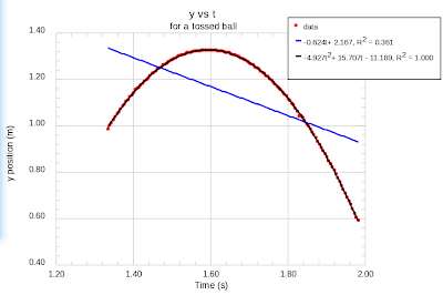
The resultant graph looks like this (after clicking the legend and title to adjust the positioning).

For the physics crowd, you will clearly see that these data originated from a ball drop and, as such, the quadratic fits much better. In fact these data result from the "Falling Motion" lab included in OpenTrack's tracking portion of the program.

A new release of OT/JSvg is due out shortly, and when it comes I will go over some of the new features.

Cheers!